spring_sensitivity

   spring_sensitivity.m

This code demonstrates the computation of sensitivities for the spring equation

$\begin{array}{l} \ddot{z} + C \dot{z} + Kz = 0 \\ \noalign{\smallskip} z(0) = 2 , \dot{z}(0) = -C \end{array}$

both by differentiating the analytic solution and approximating the solution to the sensitivity equations.

  clear all

Construct independent variables and constants.

  t = 0:.01:5;

  C = 1.5;
  K = 20.5;
  factor = sqrt(K - C^2/4);
  factor2 = sqrt(4*K - C^2);
  params = [C,K];

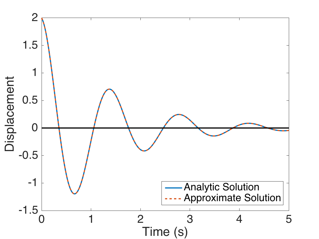
Compute analytic and approximate displacement and plot the two solutions.

  z = 2*exp(-C*t/2).*cos(factor*t);
  z0 = [2; -C];
  ode_options = odeset('RelTol',1e-8);
  [t,z_app] = ode45(@spring_rhs,t,z0,ode_options,params);

  figure(1)
  plot(t,z,t,z_app(:,1),'--',t,0*z,'k','linewidth',2)
  legend('Analytic Solution','Approximate Solution','Location','SouthEast')
  xlabel('Time (s)')
  ylabel('Displacement')
  set(gca,'Fontsize',[20]);

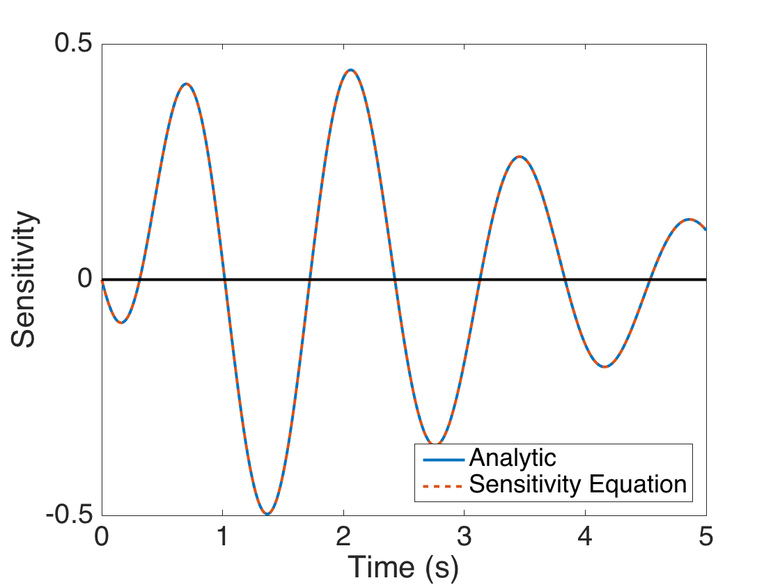
Approximate the analytic and approximate solutions to the sensitivity equations constructed for C. Plot to compare the solutions.

  zc = exp(-C*t/2).*((C*t/factor2).*sin(factor*t) - t.*cos(factor*t));
  zc0 = [0; -1];
  [t,zc_app] = ode45(@spring_sens_rhs,t,zc0,ode_options,params);

  figure(2)
  plot(t,zc,t,zc_app(:,1),'--',t,0*zc,'k','linewidth',2)
  legend('Analytic','Sensitivity Equation','Location','SouthEast')
  xlabel('Time (s)')
  ylabel('Sensitivity')
  set(gca,'Fontsize',[20]);