Example7_15_long.m

Construct synthetic data and sampling distribution for the damping parameter C as illustrated in Example 7.15. This code also constructs the density from 10,000 simulations, which is compared with the sampling distribution. Because this requires repeated optimization, the code takes approximately 40 seconds to run.

Required functions: spring_function.m ksdensity.m

  clear all
  close all

Specify true parameter and measurement variance values.

  m = 1;
  k = 20.5;
  c = 1.5;
  sigma = .1;
  var = sigma^2;

Construct synthetic data, the sensitivity matrix, and covariance matrix V.

  num = sqrt(4*m*k - c^2);
  den = 2*m;

  t = 0:.01:5;
  error = sigma*randn(size(t));
  n = length(t);

  y = 2*exp((-c/den)*t).*cos((num/den)*t);
  dydc = -(t/m).*exp((-c/den)*t).*cos((num/den)*t) + (c*t/(m*num)).*exp((-c/den)*t).*sin((num/den)*t);
  V = inv(dydc*dydc')*var;
  obs = y + error;

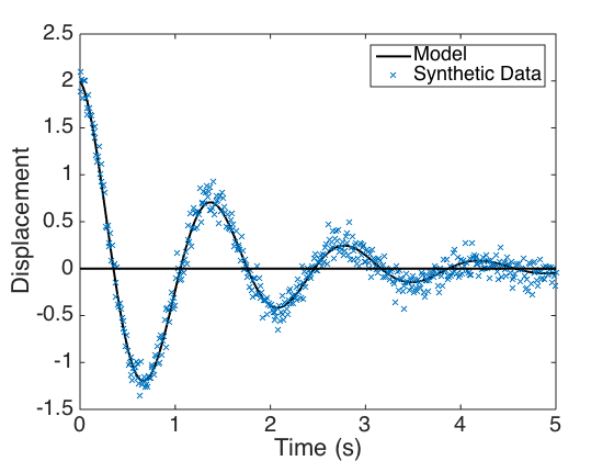
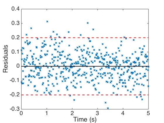
Plot the model response, synthetic data, and residuals. One notes in the residual plot that the 2 sigma interval contains approximately 95% of the residuals.

  figure(1)
  plot(t,y,'k','linewidth',2)
  hold on
  plot(t,obs,'x','linewidth',1)
  plot(t,0*y,'k','linewidth',2)
  hold off
  set(gca,'Fontsize',[20]);
  legend('Model','Synthetic Data','Location','NorthEast')
  xlabel('Time (s)')
  ylabel('Displacement')

  figure(2)
  plot(t,error,'x',t,0*y,'k','linewidth',2)
  hold on
  plot(t,2*sigma*ones(size(t)),'--r',t,-2*sigma*ones(size(t)),'--r','linewidth',2)
  hold off
  set(gca,'Fontsize',[20]);
  xlabel('Time (s)')
  ylabel('Residuals')

Construct sampling distribution and determine optimal value of C using the routine fminsearch.m for this data. We additionally compute the confidence interval.

  C = [1.4:.001:1.6];
  sample_dist = normpdf(C,1.5,sqrt(V));

  modelfun = @(c) spring_function(c,m,k,obs,t);
  [c_opt,fval] = fminsearch(modelfun,c);

  c_opt
  conf_int = [c_opt - 1.96*sqrt(V) c_opt + 1.96*sqrt(V)]

c_opt =

    1.4512


conf_int =

    1.4154    1.4871

Construct the density by repeated sampling. The final KDE is performed using ksdensity. The variable count compiles the number of 95% confidence intervals that contain the true parameter value.

  count = 0;
  for j = 1:10000
    error = sigma*randn(size(t));
    y = 2*exp((-c/den)*t).*cos((num/den)*t);
    obs = y + error;
    modelfun = @(c) spring_function(c,m,k,obs,t);
    [c_opt,fval] = fminsearch(modelfun,c);
    c_lower = c_opt - 1.96*sqrt(V);
    c_upper = c_opt + 1.96*sqrt(V);
    if (c_lower <= c) & (c <= c_upper)
      count = count + 1;
    end
    Cvals(j) = c_opt;
  end
  count

  [density_C,Cmesh] = ksdensity(Cvals);

count =

        9510

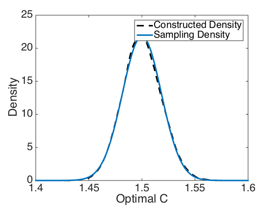
Plot the sampling distribution and constructed density computed by generating data and optimizing 10,000 times.

  ylabel('Residuals')

  figure(3)
  plot(Cmesh,density_C,'k--','linewidth',3)
  axis([1.4 1.6 0 25])
  hold on
  plot(C,sample_dist,'linewidth',3)
  set(gca,'Fontsize',[22]);
  xlabel('Optimal C')
  ylabel('Density')
  legend('Constructed Density','Sampling Density','Location','NorthEast')

Published with MATLAB® R2014b