Example10

                Example10_13.m

Compute the mean and standard deviation of the steady state spring solution

$y(\omega_F,Q) = \frac{1}{\sqrt((k-m \omega_F^2)^2 + (c\omega_F)^2}$

with coefficients Q = [m,c,k].  Here we compare three methods:
 * Monte Carlo sampling as discussed in Section 9.2 with mean and variance at omega_f given by (9.20)
 * Deterministic solutions y(omega_F,\bar{q})
 * Discrete projection

  clear all

%
%

  K = 9;           % Number of tensored Hermite basis functions Psi(q)
  N_MC = 1e5;      % Number of Monte Carlo samples
  M = 10;          % Number of Gauss-Hermite quadrature points used to approximate discrete projection

Input the parameter means and standard deviations.

  mu_m = 2.7;
  mu_c = 0.24;
  mu_k = 8.5;
  sigma_m = 0.002;
  sigma_c = 0.065;
  sigma_k = 0.001;

Compute N_MC samples for each of the parameters and construct the grid for omega_F.

  q = zeros(N_MC,3);
  q(:,1) = mu_m + sigma_m*randn(N_MC,1);
  q(:,2) = mu_c + sigma_c*randn(N_MC,1);
  q(:,3) = mu_k + sigma_k*randn(N_MC,1);

  d_omega = 0.005;
  omega = [0.5:d_omega:2.7];
  N_omega = length(omega);

Input the M=10 Gauss-Hermite quadrature points and weights from a table.

  zvals = sqrt(2)*[-3.4361 -2.5327 -1.7566 -1.0366 -0.3429 0.3429 1.0366 1.7566 2.5327 3.4361];
  weights = (1/sqrt(pi))*[7.6404e-6 1.3436e-3 3.3874e-2 2.4014e-1 6.1086e-1 6.1086e-1 2.4014e-1 3.3874e-2 1.3436e-3 7.6404e-6];

  mvals = mu_m*ones(size(zvals)) + sigma_m*zvals;
  cvals = mu_c*ones(size(zvals)) + sigma_c*zvals;
  kvals = mu_k*ones(size(zvals)) + sigma_k*zvals;

Constuct the Hermite polynomials H_0, H_1 and H_2 evaluated at the quadrature points zvals. Also construct the coefficients h0, h1 and h2 used to construct gamma_k.

  poly0 = ones(1,M);                  % H_0(q) = 1
  poly1 = zvals;                      % H_1(q) = q
  poly2 = zvals.^2 - ones(1,M);       % H_2(q) = q^2 - 1
  h0 = factorial(0);
  h1 = factorial(1);
  h2 = factorial(2);

  y_k0 = zeros(1,N_omega);
  y_k1 = zeros(1,N_omega);
  y_k2 = zeros(1,N_omega);
  y_k3 = zeros(1,N_omega);
  y_k4 = zeros(1,N_omega);
  y_k5 = zeros(1,N_omega);
  y_k6 = zeros(1,N_omega);
  y_k7 = zeros(1,N_omega);
  y_k8 = zeros(1,N_omega);
  y_k9 = zeros(1,N_omega);

Compute the deterministic, Monte Carlo and discrete projection values at each of values omega_F.

  for k = 1:N_omega
    deterministic(k) = 1/sqrt((mu_k-mu_m*omega(k)^2)^2 + (mu_c*omega(k))^2);     % Deterministic solution
    MC = 1./sqrt((q(:,3)-q(:,1)*omega(k)^2).^2 + (q(:,2)*omega(k)).^2);          % Monte Carlo samples
    MC_mean(k) = (1/N_MC)*sum(MC);                                               % MC mean
    tmp = 0;
    for j=1:N_MC
       tmp = tmp + (MC(j) - MC_mean(k))^2;
    end
    MC_sigma(k) = sqrt((1/(N_MC-1))*tmp);

    for j1 = 1:M
      for j2 = 1:M
        for j3 = 1:M
          denom = (kvals(j2) - mvals(j1)*omega(k)^2)^2 + (cvals(j3)*omega(k))^2;
          yval = 1/sqrt(denom);
          y_k0(k) = y_k0(k) + (1/(h0*h0*h0))*yval*poly0(j1)*poly0(j2)*poly0(j3)*weights(j1)*weights(j2)*weights(j3);
          y_k1(k) = y_k1(k) + (1/(h1*h0*h0))*yval*poly1(j1)*poly0(j2)*poly0(j3)*weights(j1)*weights(j2)*weights(j3);
          y_k2(k) = y_k2(k) + (1/(h0*h1*h0))*yval*poly0(j1)*poly1(j2)*poly0(j3)*weights(j1)*weights(j2)*weights(j3);
          y_k3(k) = y_k3(k) + (1/(h0*h0*h1))*yval*poly0(j1)*poly0(j2)*poly1(j3)*weights(j1)*weights(j2)*weights(j3);
          y_k4(k) = y_k4(k) + (1/(h2*h0*h0))*yval*poly2(j1)*poly0(j2)*poly0(j3)*weights(j1)*weights(j2)*weights(j3);
          y_k5(k) = y_k5(k) + (1/(h1*h1*h0))*yval*poly1(j1)*poly1(j2)*poly0(j3)*weights(j1)*weights(j2)*weights(j3);
          y_k6(k) = y_k6(k) + (1/(h1*h0*h1))*yval*poly1(j1)*poly0(j2)*poly1(j3)*weights(j1)*weights(j2)*weights(j3);
          y_k7(k) = y_k7(k) + (1/(h0*h2*h0))*yval*poly0(j1)*poly2(j2)*poly0(j3)*weights(j1)*weights(j2)*weights(j3);
          y_k8(k) = y_k8(k) + (1/(h0*h1*h1))*yval*poly0(j1)*poly1(j2)*poly1(j3)*weights(j1)*weights(j2)*weights(j3);
          y_k9(k) = y_k9(k) + (1/(h0*h0*h2))*yval*poly0(j1)*poly0(j2)*poly2(j3)*weights(j1)*weights(j2)*weights(j3);
        end
      end
    end
  end

Compute the mean and variance based on the generalized Fourier coefficients y_k.

  Y_k = [y_k0; y_k1; y_k2; y_k3; y_k4; y_k5; y_k6; y_k7; y_k8; y_k9];
  gamma = [h0*h0*h0 h1*h0*h0 h0*h1*h0 h0*h0*h1 h2*h0*h0 h1*h1*h0 h1*h0*h1 h0*h2*h0 h0*h1*h1 h0*h0*h2];

  for n = 1:N_omega
    var_sum = 0;
    for j = 2:K+1
      var_sum = var_sum + (Y_k(j,n)^2)*gamma(j);
    end
    var(n) = var_sum;
  end

  DP_mean = Y_k(1,:);           % Discrete projection mean
  DP_sd = sqrt(var);            % Discrete projection standard deviation

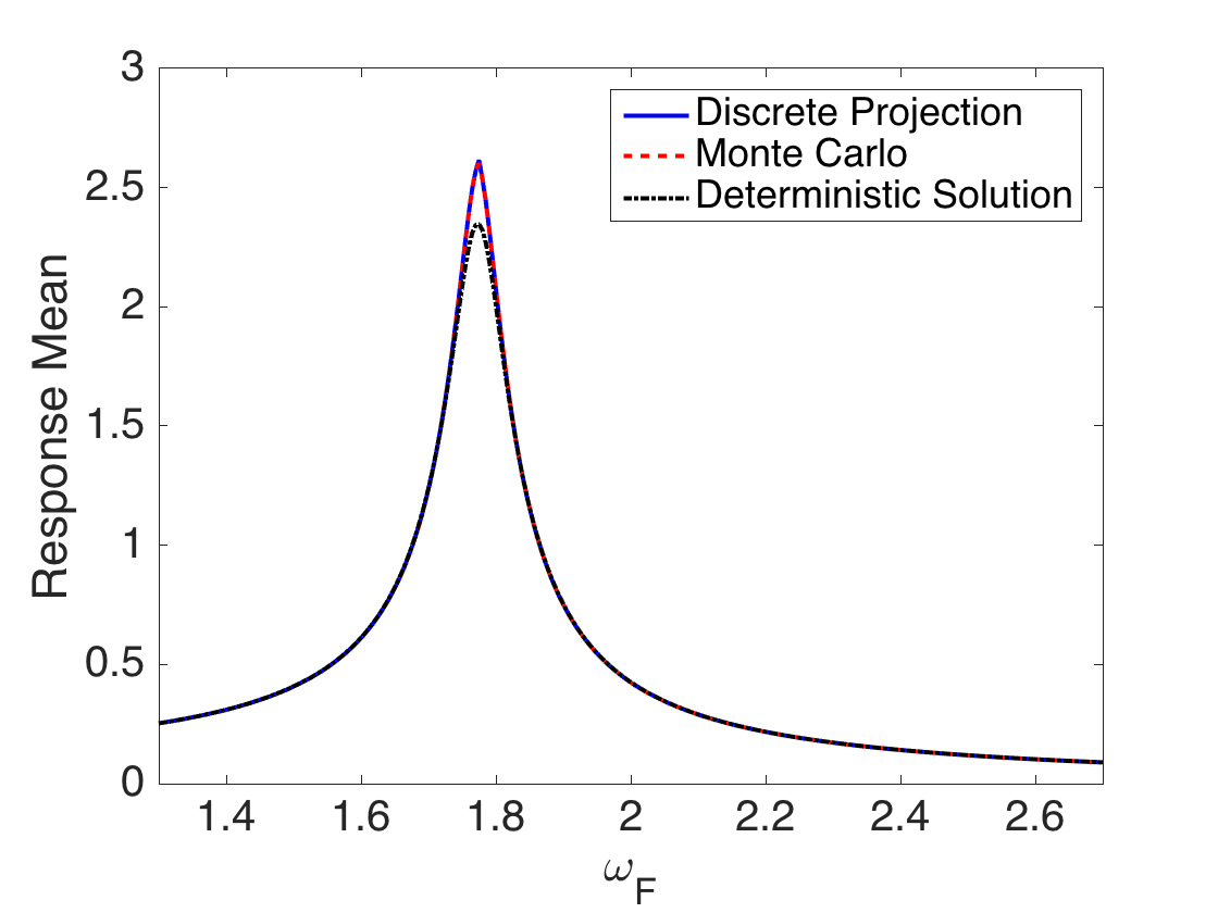
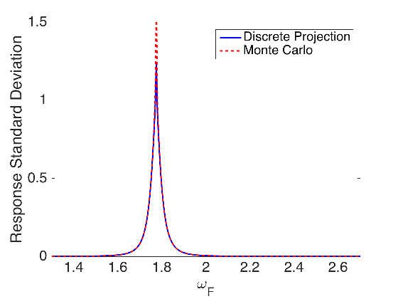
Plot the response mean and standard deviation as a function of the drive frequency omega_F.

  figure(1)
  plot(omega,DP_mean,'b-',omega,MC_mean,'--r',omega,deterministic,'-.k','linewidth',2)
  axis([1.3 2.7 0 3])
  set(gca,'Fontsize',[20]);
  xlabel('\omega_F')
  ylabel('Response Mean')
  legend('Discrete Projection','Monte Carlo','Deterministic Solution','Location','NorthEast')


  figure(2)
  plot(omega,DP_sd,'-b',omega,MC_sigma,'--r','linewidth',2)
  axis([1.3 2.7 0 1.5])
  set(gca,'Fontsize',[20]);
  xlabel('\omega_F')
  ylabel('Response Standard Deviation')
  legend('Discrete Projection','Monte Carlo','Location','NorthEast')